GEARS Explained: How Graph Neural Networks Predict the Unseen

A deep dive into the model that can forecast what happens when you knock out genes nobody has ever touched.

The Problem

You’re a biologist. You have a Perturb-seq dataset — 100,000 cells, each with one or two genes CRISPR-knocked out, plus single-cell RNA-seq readouts of the full transcriptome. You’ve experimentally perturbed 100 single genes and 130 two-gene combos. But there are 4,950 untested pairwise combinations. Running them all would cost a fortune.

Can a model trained on 230 experiments predict the other 4,950?

And harder still: can it predict the effect of perturbing a gene that was never experimentally perturbed at all?

This is the problem GEARS solves.

What GEARS Is

GEARS — Graph-Enhanced gene Activation and Repression Simulator — is a deep learning model from Stanford’s SNAP Lab (Roohani, Huang & Leskovec, Nature Biotechnology, 2023). It predicts the transcriptional outcome of single and multi-gene perturbations using single-cell RNA-seq data.

The architecture is deceptively simple. Here it is, from Figure 1 of the paper:

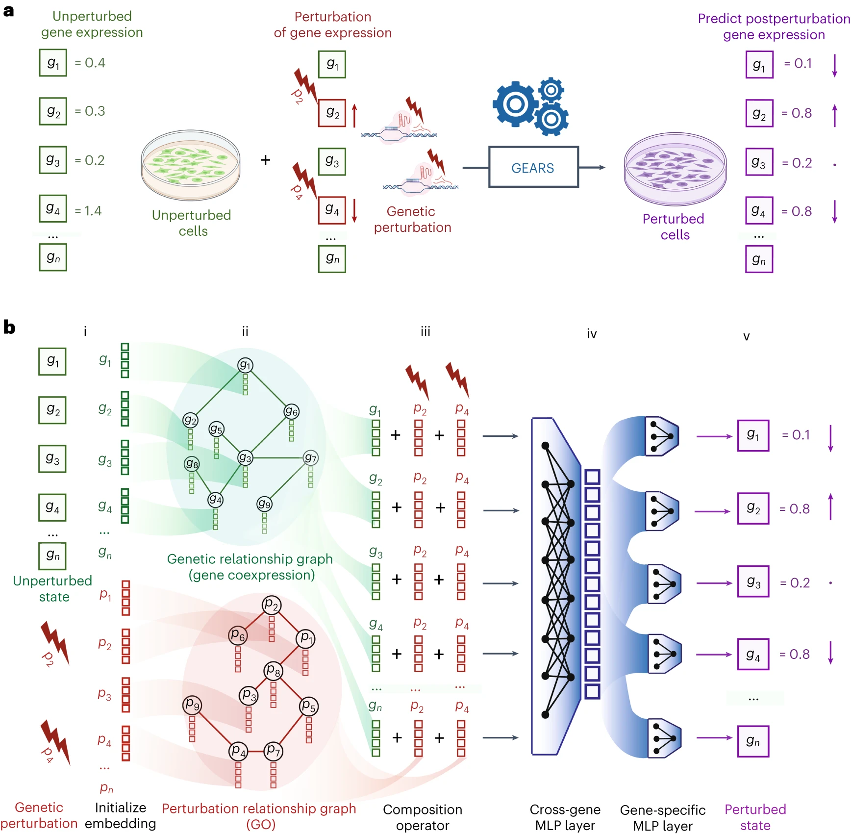
a, Problem formulation: given unperturbed gene expression (green) and applied perturbation (red), predict the gene expression outcome (purple). Each box corresponds to an individual gene. Arrows indicate change in expression. b, GEARS model architecture. (i) For each gene in the unperturbed state, GEARS initializes a gene embedding vector (green) and a gene perturbation embedding vector (red) (ii). These embedding vectors are assigned as node features in the gene relationship graph and the perturbation relationship graph (iii). A GNN is used to combine information between neighbors in each graph. Each resulting gene embedding is summed with the perturbation embedding of each perturbation in the perturbation set (iv). The output is combined across all genes using the cross-gene layer and fed into gene-specific output layers (v). The final result is postperturbation gene expression; MLP, multilayer perceptron.

Input: the gene expression of a control cell + which genes are being perturbed.
Output: the gene expression of the cell after perturbation.

Under the hood, five components work in sequence. Let me walk through each one.

The Five Components

Component 0: Two Knowledge Graphs (Built Before Training)

Before the neural network sees a single data point, GEARS constructs two graphs. These are the secret sauce — they give the model its zero-shot capability.

Graph A: The Co-expression Graph

Built from the training data. For every pair of genes, compute the Pearson correlation of their expression across all control cells. Keep the top-20 most correlated neighbors per gene (above a 0.4 threshold). Edge weight = the absolute correlation coefficient.

What it captures: “BRCA1 and BRCA2 are always up or down together, so they probably respond similarly to perturbations.”

Graph B: The Gene Ontology (GO) Graph

Built from the GO database — a human-curated catalog of which genes participate in which biological processes. Edge weight = Jaccard similarity of shared GO terms. Keep edges above 0.1 similarity, top-20 neighbors per gene.

What it captures: “BRCA1 and RAD51 both participate in DNA repair, so knocking out one probably has similar downstream effects to knocking out the other.”

These graphs are frozen during training. Their weights never change. They serve as fixed wiring that tells the GNN layers which genes should talk to each other.

Component 1: Gene Embeddings + Co-expression GNN

Every gene gets a learnable 64-dimensional vector — its gene embedding (gene_emb). Initially random numbers, these vectors are gradually shaped by backpropagation to encode each gene’s properties.

A second embedding table (emb_pos) runs through a Simple Graph Convolution (SGConv) on the co-expression graph:

pos_emb_new[BRCA1] = 0.92 × pos_emb[BRCA2] + 0.78 × pos_emb[TP53] + ...

This is a weighted average of neighbors’ embeddings. After each GNN layer, co-expressed genes have more similar position embeddings.

The final gene representation merges both:

base_emb[gene] = gene_emb[gene] + 0.2 × GNN(emb_pos[gene])

The 0.2 coefficient ensures the GNN provides a whisper, not a shout — preserving each gene’s uniqueness while adding relationship context.

Component 2: Perturbation Embeddings + GO GNN

Every gene that can be perturbed gets a separate perturbation embedding (pert_emb), also 64-dimensional. This is not the same as the gene embedding — it represents “what happens when you perturb this gene.”

This embedding runs through SGConv on the GO graph:

pert_emb_new[TP53] = 0.6 × pert_emb[BRCA1] + 0.5 × pert_emb[CHEK2] + ...

This is where zero-shot prediction is born. Even if TP53 was never experimentally perturbed, its perturbation embedding is a weighted blend of functionally similar genes (like BRCA1 and CHEK2) that were perturbed. During training, gradients from BRCA1’s data “leak” across the GO edge to TP53’s embedding, giving it a meaningful value despite zero direct training examples.

Component 3: The Composition Module — Broadcasting Perturbation Information

Here’s where things get interesting. For each cell in a batch:

# Sum perturbation embeddings for all perturbed genes in this cell
pert_sum = pert_emb[BRCA1] + pert_emb[TP53]

# Run through an MLP to allow non-additive interactions
pert_fused = MLP(pert_sum)   # pert_fuse: 64 → 64 → 64

# Add the SAME vector to EVERY gene in this cell
for gene in all_genes:
    base_emb[gene] += pert_fused

Key design decision: the perturbation signal is broadcast identically to all genes. Not weighted by distance in the GO graph, not targeted to specific genes — every gene receives the same 64-dimensional “this cell is being perturbed” signal.

Why? Because a knocked-out transcription factor can affect thousands of target genes across diverse pathways. Constraining the signal by GO similarity would miss these distal effects. Instead, GEARS lets each gene decide for itself how much to respond, through the next component.

The pert_fuse MLP is critical: it takes the simple sum of two perturbation embeddings and applies a nonlinear transformation. Without it, double perturbations would be purely additive. With it, the model can learn that BRCA1+TP53 is synergistic (1+1=10) or antagonistic (1+1=0.3).

Component 4: Gene-Specific Decoder — Every Gene Has Its Own Weights

After a recovery MLP that cross-mixes the 64 dimensions, the representation hits the gene-specific decoder:

# For each gene:
prediction[gene_i] = dot_product(base_emb[gene_i], indv_w1[gene_i]) + indv_b1[gene_i]

indv_w1 is a (num_genes × 64 × 1) parameter — each gene has 64 weights and 1 bias. No sharing.

This is not a neural network layer. It’s a linear dot product. But having per-gene parameters means:

Housekeeping genes (like ACTB) learn weights near zero plus a bias near the baseline expression — perturbations barely affect them.
Transcription factor targets learn large weights on dimensions carrying perturbation signals — they change dramatically.
The model never needs to learn a “one-size-fits-all” mapping from perturbation signal to expression change — each gene has its own translation table.

Component 5: The Cross-Gene Layer — Whole-Cell Awareness

After the gene-specific decoder, we have one scalar prediction per gene — but each gene made its prediction in isolation, unaware of what other genes are doing.

The cross-gene MLP fixes this:

# Input: all 5,000 genes' local predictions → compress to 64-dim global state
global_state = MLP([local_pred_gene0, local_pred_gene1, ..., local_pred_gene4999])
# MLP: 5000 → 64 → 64

# Broadcast back to every gene
for gene in all_genes:
    combined_input = [local_pred[gene], global_state]
    final_delta[gene] = dot_product(combined_input, indv_w2[gene]) + indv_b2[gene]

Each gene’s final prediction now combines:

Local information: its own direct response to the perturbation
Global information: the emergent state of the entire transcriptome

The 5000→64 compression is aggressive (~80:1), but it forces the model to extract a meaningful summary: “is this cell in apoptosis?” or “is this cell proliferating?” — emergent properties that no single gene captures alone.

The Residual Connection

final_expression = delta + x_control

The entire pipeline above computes delta — the change from baseline. Adding back the control expression means:

If the model learns nothing (delta ≈ 0), the output is the control expression — a reasonable default.
The model focuses on learning differences, not memorizing baseline expression levels.
Gradient flow is improved: the input has a direct path to the output.

How It Learns: The Loss Function

GEARS uses a two-part loss:

Loss = MSE_weighted + direction_lambda × Direction_Loss

Weighted MSE: (pred - true)^(2+gamma) with gamma=2, meaning (pred - true)^4. Errors on highly-expressed genes are punished disproportionately — getting a 10-fold-change gene wrong by 1.0 matters more than getting a 0.1-expression gene wrong by 1.0.

Direction Loss: (sign(pred - control) - sign(true - control))^2. If the real gene went up and the model predicted down, this penalty kicks in hard (value of 4). If both went up, zero penalty — the MSE handles the magnitude. This is biologically critical: confusing activation for repression is a fundamental misinterpretation of the regulatory relationship.

How It’s Evaluated

Data Split Strategy

GEARS uses a simulation split to test generalization:

All perturbation genes (e.g., 131 genes)
    │
    ├── 75% "seen" (train) — 98 genes
    │   ├── Single perturbations → training
    │   └── Combo perturbations → 75% train, 25% test
    │
    └── 25% "unseen" (test) — 33 genes
        ├── Single perturbations → test (unseen_single)
        ├── Combo: both unseen (combo_seen0)
        └── Combo: one seen + one unseen (combo_seen1)

This mirrors real-world use: you’ve perturbed some genes, now predict the rest.

Metrics

MSE_de: Mean squared error on the top 20 differentially expressed genes. The hardest metric — these genes change the most and are most biologically important.
Pearson correlation: Overall agreement between predicted and true expression.
Direction accuracy: Fraction of top-20 DE genes where the sign matches reality.
Precision@10 (for GI): Among the top-10 predicted strongest interactions, what fraction are real?

Baselines

GEARS is compared against:

No-perturbation baseline: assume the perturbation changes nothing (delta = 0 everywhere)
CPA (Lotfollahi et al.): prior deep learning method without knowledge graphs
Gene regulatory network propagation (CellOracle-style): infer a GRN, linearly propagate perturbation effects along edges

The Training Loop

for epoch in range(epochs):
    for batch in train_loader:
        pred = model(batch)               # forward pass
        loss = loss_fct(pred, batch.y)    # weighted MSE + direction loss
        loss.backward()                   # gradients
        clip_grad_norm_(1.0)             # prevent explosions
        optimizer.step()                  # update all parameters

    # Evaluate on validation set
    val_metrics = evaluate(val_loader)
    if val_metrics['mse_de'] < best_val:
        best_model = deepcopy(model)     # checkpoint

    scheduler.step()                     # learning rate decay

Key training details:

Adam optimizer with weight decay
Gradient clipping at 1.0
StepLR scheduler: learning rate halves periodically
Early stopping: keep the model with best validation MSE_de
Training on 1,543 perturbations (~170K cells) takes ~20 epochs

Where Backpropagation Flows

Every trainable parameter gets gradients from the loss through the chain rule:

Loss
  ↓ ∂L/∂y_pred
Residual connection (+x)
  ↓ ∂L/∂delta
indv_w2, indv_b2  ← per-gene weights updated
  ↓
Cross-gene MLP   ← global state weights updated, gradients flow between genes
  ↓
indv_w1, indv_b1  ← per-gene weights updated
  ↓
Recovery MLP     ← W1, W2, b1, b2 updated
  ↓
Gene embedding   ← gene_emb and emb_pos updated
  ↓
Perturbation embedding ← pert_emb updated
  ↓
SGConv layers    ← Linear weights updated; gradients flow along GO/coexpr edges

The GNN layers are the critical bridge: gradients from data-rich genes propagate across graph edges to data-poor neighbors, giving them meaningful embeddings despite zero direct supervision.

Why Five Components Work Together

Component	Role	Without It
Co-expression GNN	“Genes that express together respond together”	Cannot exploit expression patterns
GO GNN	“Functionally similar genes perturb similarly”	Zero-shot prediction impossible
Broadcast + pert_fuse	“Every gene knows the perturbation; MLP enables non-additivity”	Only additive combo predictions
Gene-specific decoder	“Each gene has unique regulatory logic”	One-size-fits-none predictions
Cross-gene MLP	“Genes coordinate; cell state matters”	No emergent phenotype detection
Residual connection	“Learn changes, not absolutes”	Must memorize baselines

The result: 40% higher precision than prior methods in predicting genetic interactions, >30% MSE reduction for single-gene perturbation prediction, and the ability to predict entirely novel phenotypes that were never seen in training data.

What GEARS Cannot Do (Yet)

Cross-cell-type transfer: Train on K562, predict on RPE-1 — not supported. Each model is cell-type-specific.
Temporal dynamics: Predicts only the steady-state post-perturbation expression, not the trajectory.
Perturbation strength: Binary (perturbed/not perturbed), not dose-dependent.
>2 gene combos: Trained and tested primarily on single and double perturbations.
Bulk RNA-seq: Designed for single-cell data with many cells per perturbation.

Every one of these limitations has spawned follow-up work (TxPert, Dango, SCALE, AlphaCell, HyperMap — see the rapidly growing citation tree).

References

Roohani, Y., Huang, K. & Leskovec, J. Predicting transcriptional outcomes of novel multigene perturbations with GEARS. Nature Biotechnology 42, 927–935 (2024).
GitHub: snap-stanford/GEARS

The Problem#

What GEARS Is#

The Five Components#

Component 0: Two Knowledge Graphs (Built Before Training)#

Component 1: Gene Embeddings + Co-expression GNN#

Component 2: Perturbation Embeddings + GO GNN#

Component 3: The Composition Module — Broadcasting Perturbation Information#

Component 4: Gene-Specific Decoder — Every Gene Has Its Own Weights#

Component 5: The Cross-Gene Layer — Whole-Cell Awareness#

The Residual Connection#

How It Learns: The Loss Function#

How It’s Evaluated#

Data Split Strategy#

Metrics#

Baselines#

The Training Loop#

Where Backpropagation Flows#

Why Five Components Work Together#

What GEARS Cannot Do (Yet)#

References#